Introduction

High water events such as storm surge, riverine flooding, or high-tide flooding can inundate a stormwater network and reduce its effectiveness.

bathtub is an R package that estimates the impact of downstream flooding on stormwater infrastructure using a simple bathtub model and a 1-dimensional model of the stormwater network.

bathtub is not designed to replace more complex hydrodynamic modeling (e.g., SWMM), but rather to be a simpler and more accessible option for estimating potential impacts of inundation of stormwater networks.

To use bathtub, you must have spatial data representing the stormwater network, and these data must include information representing the elevation or depth of stormwater inverts.

The following tutorial will use data from Beaufort, North Carolina to present the workflow for bathtub, which consists of:

• Managing data
• Creating a bathtub model
• Running the model
• Visualizing results
• Loading/sharing models & results

Managing Data

bathtub saves models and model results as geopackages so you can load them later or share them.

The first step is to create the output folder and set the workspace for the project.

Setting up the workspace

Run folder_setup() to create the folders needed for bathtub and produce the workspace path. bathtub uses the provided path to create a bathtub_output folder with five subfolders:

• DEMs (digital elevation models)
• figures
• input
• model
• results

library(bathtub)

workspace <- folder_setup("your_path_here")
site_name <- "beaufort"

Load network data

Next step is to load the stormwater network spatial data. I’ve put the spatial network data into the bathtub_output/input folder so I can easily share it later.

In this example, invert elevations are calculated ahead of time using surveyed invert depth and elevation.

Different structure types (i.e., pipe ends, junction boxes, etc.) have their own shapefiles, but we need to combine them into one structures object.

library(sf)
library(mapview)
library(tidyverse)

#> read in pipes shapefile, but I don't want any 'pipes' that are classified as 'shoreline'
pipes <- st_read(paste0(workspace,"/input/bft_storm_lines_subset.shp")) %>%
  st_zm() %>%
  filter(!NOTES %in% "shoreline")

#> read in structure shapefiles, calculate Invert elevations, and reproject to the same projection (crs) as pipes
pipe_ends <- st_read(paste0(workspace,"/input/pipe_ends.shp")) %>%
  st_zm() %>%
  mutate(INVERTELEV = Elevation - Out1_Dpth) %>%
  dplyr::select(Elevation, INVERTELEV, Code, Prcnt_Obst, Type_Obst) %>%
  st_transform(crs = st_crs(pipes))

junction_boxes <- st_read(paste0(workspace,"/input/junction_boxes.shp")) %>%
  st_zm()%>%
  mutate(INVERTELEV = if_else(Out1_Dpth != 0, Elevation - Out1_Dpth, 99)) %>%
  dplyr::select(Elevation, INVERTELEV, Code, Prcnt_Obst, Type_Obst)%>%
  st_transform(crs = st_crs(pipes))

drop_inlets <- st_read(paste0(workspace,"/input/drop_inlets.shp")) %>%
  st_zm()%>%
  mutate(INVERTELEV = Elevation - Out1_Dpth) %>%
  dplyr::select(Elevation, INVERTELEV, Code,Prcnt_Obst, Type_Obst)%>%
  st_transform(crs = st_crs(pipes))

catch_basins <- st_read(paste0(workspace,"/input/catch_basins.shp")) %>%
  st_zm()%>%
  mutate(INVERTELEV = Elevation - Out1_Dpth) %>%
  dplyr::select(Elevation, INVERTELEV, Code,Prcnt_Obst, Type_Obst)%>%
  st_transform(crs = st_crs(pipes))

#> Not all structures were surveyed, but 'bathtub' will conservatively estimate invert elevations based on known invert elevations connected to them
unknown_structures <- st_read(paste0(workspace,"/input/unknown_elevs_sub.shp")) %>%
  st_zm() %>%
  mutate(Elevation = NA,
         INVERTELEV = NA,
         Code = TYPE_FEAT,
         Prcnt_Obst = NA,
         Type_Obst = NA) %>%
  dplyr::select(Elevation, INVERTELEV, Code, Prcnt_Obst, Type_Obst) %>%
  st_transform(crs = st_crs(pipes))

#> combine all structures into one 'sf' object using rbind. Note that I made all structures have the same column structure
structures <- rbind(pipe_ends,
                    junction_boxes,
                    drop_inlets,
                    catch_basins,
                    unknown_structures)

Load elevation data

bathtub comes with a conversion raster to convert NAVD88 to the mean higher high water (MHHW) tidal datum in North Carolina.

Load this conversion raster and download elevation data for the study area using get_NOAA_elevation().

get_NOAA_elevation() uses the extent of the pipe layer (plus a small buffer) to download NOAA elevation data that is made for sea level rise inundation mapping.

#> read in conversion rasters for NAVD88 --> MHHW
NAVD88_MHHW <- bathtub::NAVD88_MHHW_NC

#> Download NOAA SLR DEM. Native res is ~3m. We'll request 10ft. 
noaa_elev <- bathtub::get_NOAA_elevation(x = pipes,
                                x_EPSG = 102719,
                                res = 10,
                                workspace = workspace)

Model setup

This step converts all input data to the correct spatial projection and units.

Set up elevation

bathtub uses the tidal datum of mean higher high water (MHHW) for inundation modeling, so we must convert the downloaded elevation data from NAVD88 to MHHW.

The converted DEM will be saved in bathtub_output/DEMs/.

DEM_setup() also clips elevation data to the study area for faster processing. If you have previously run DEM_setup(), you can set overwrite to FALSE, and the previous result will be loaded.

#> Convert elevation to MHHW
bft_elev <-
  DEM_setup(
    pipes = pipes,
    large_DEM = noaa_elev,
    conversion_raster = NAVD88_MHHW,
    res = 10,
    trace_upstream = F,
    workspace = workspace,
    overwrite = T
  )

Set up pipes & structures

This step structures the pipe and structure data with units and defines the column names that the model will use.

In this case, all stormwater network elevation data is stored in the structures layer, so type = "none". If elevation or depth data were stored in the pipe layer, type = "elevation" or type = "depth", respectively.

#> Setup pipes and structures with units. Uses surveyed surface & invert elevations
pipes_n <-
  setup_pipes(pipes,
              type = "none",
              diam = "DIAMETER",
              diam_units = "in")

#> These functions also allow null values to be declared. Shapefiles can't store "NA" values, so the null values will be converted from a number to NA. 
structures_n <-
  setup_structures(
    structures = structures,
    type = "elevation",
    invert = "INVERTELEV",
    elev = "Elevation",
    elev_units = "ft",
    null_value = 99,
    other_cols = c("Code","Prcnt_Obst","Type_Obst"),
    workspace = workspace
  )

Assemble model

Using properly structured pipe and structure data, we create the model using assemble_net_model().

assemble_net_model():

• identifies connectivity between pipes and structures
• interpolates missing invert elevations up/down the network
• automatically identifies outlets

The output model consists of 3 sf objects:

• Pipes
• Nodes (ends of pipes)
• Structures

Each object is written to bathtub_output/model/ along with a file for each object that describes the units of each column (see save_w_units() function).

All connectivity information is stored in the ‘nodes’ layer.

bft_model<- assemble_net_model(
  pipes = pipes_n,
  structures = structures_n,
  type = "none",
  elev = bft_elev,
  elev_units = "m",
  use_raster_elevation = F,
  buffer = 1,
  guess_connectivity = T,
  workspace = workspace
)

Run the model

bathtub can model impacts using: - a range of water levels - spatial data showing extent of flooding - time series of downstream water level (in development)

This example shows how to run the model using a range of water levels, from -3 ft MHHW to 4 ft MHHW by 3 inch increments.

We’re also interested in flooding hotspots caused by stormwater network surcharge, so model_ponding is set to TRUE. If you are modeling a large area or lots of model steps, start with model_ponding = F.

All model results are written (along with their associated unit files) to bathtub_output/results/.

Model results consist of:

• impacted features (pipes, nodes, structures) with propagation through stormwater network,
• impacted features (np_nodes, np_structures) with no propagation (i.e., only overland flooding)
• flooding extent, and
• ponding extent (if model_ponding = T)

for each modeled water level (or input flooding extent).

bft_model_output <- model_inundation(
  model = bft_model,
  elev = bft_elev,
  elev_units = "m",
  from_elevation = -3,
  to_elevation = 4,
  step = 3/12,
  model_ponding = T,
  site_name = "beaufort",
  overwrite = T,
  minimum_area = 0.01,
  workspace = workspace
)

Visualizing results

Plots

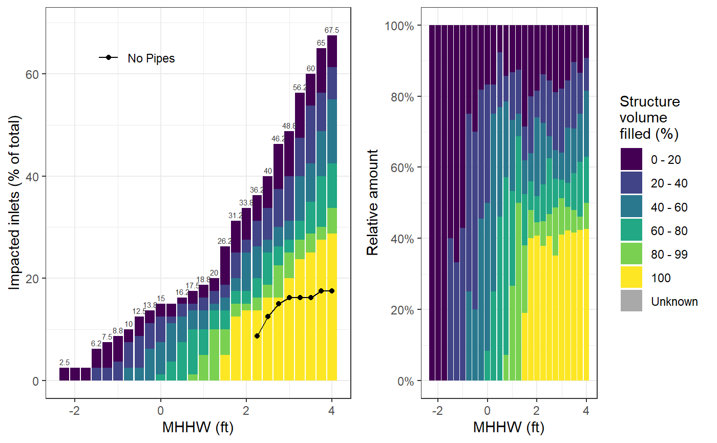
Plot the impact of inundation (percent of object filled) of structures (viz_structures()) or nodes (viz_nodes()) using the type = "plot" argument. The model results are compared to simple overland flooding impacts.

Save the plot to bathtub_output/figures/ by specifying a filename.

bft_plot <- viz_structures(model_output = bft_model_output,
                           model = bft_model,
                           elev = bft_elev,
                           type_column = "Code",
                           filter_value = "D_I",
                           type = "plot",
                           # hide_labels = T,
                           # simplify_labels = T,
                           # label_size = 2,
                           # filename = "bft_structures_impact_plot.png",
                           workspace = workspace)

bft_plot

Interactive maps

Visualize the minimum water level of impact for all structures, and click on the points to see a plot of percent fill vs. water level! This can take awhile for large models.

bft_int_structures_map <- viz_structures(model_output = bft_model_output,
                          model = bft_model,
                           elev = bft_elev,
                           type = "interactive_map",
                           workspace = workspace)
bft_int_structures_map

Use the mapview package

Results are simply a list of sf objects, so you can easily view them using the mapview package.

If viewing an attribute that is a units object, use units::drop_units() to remove units before passing the attribute name to zcol in mapview()

mapview(bft_model_output$ponding %>%
             arrange(-water_elevation),
        zcol="water_elevation",
        layer.name = "Ponding water level (ft MHHW)")

Loading & sharing models & results

Loading previous results

Model objects and results are automatically written to their respective folders within bathtub_output when they are created.

Use load_model() to re-load a model from file

Use load_results() to re-load model results file

Both of these functions only require the workspace path and also read the associated unit files to preserve units.

Sharing models & results

Share models and results by simply sharing the bathtub_output folder.

This will also share the elevation data, input data (if stored manually in the input folder), and any figures created and saved with viz_nodes() or viz_structures().

To run the bathtub model or view results, a user simply needs to set the workspace path to the bathtub_output folder.